2D Finite Element Analysis Solver
Developed a custom two-dimensional finite element analysis solver in Python to analyze the displacement, strain, and stress response of linear-elastic structures.
Project Overview
The program was built from the underlying finite element formulation rather than relying on an existing FEA library, providing direct implementation of element stiffness calculations, numerical integration, global matrix assembly, boundary conditions, loading, and stress recovery.
The solver uses four-node bilinear quadrilateral (Q4) elements and supports arbitrary element geometries and multi-element meshes. SymPy was used extensively to implement the mathematical formulation while maintaining a direct connection between the governing finite element equations and their computational implementation.
Abaqus/Standard was subsequently used as an independent commercial FEA reference to verify the custom solver through mesh-refinement studies.
Input
Finite Element Formulation
The solver implements a two-dimensional linear-elastic, plane-strain formulation. Each Q4 element uses bilinear isoparametric shape functions to interpolate the displacement field,
u = Nd,
with the strain-displacement relationship obtained from
𝜖 = Bd.
The Jacobian transformation maps derivatives of the shape functions from the element's natural coordinates (ξ, η) into the global x-y coordinate system, allowing the same element formulation to be applied to general quadrilateral geometries.
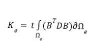
Element stiffness is calculated from
,
where t is the out-of-plane thickness, and D is the plane-strain constitutive matrix. The integral is evaluated numerically using a 2-Gaussian quadrature scheme.
Individual element matrices are then assembled into the global stiffness system,
KU = R,
which is partitioned according to prescribed and unknown degrees of freedom and solved for the global displacement field.
After solving for the nodal displacements, each element's displacement vector is extracted from the global solution. Strain is recovered from
𝜖
and stress is calculated from the constitutive relationship
σ = D𝜖
Stress and strain are evaluated at the element’s Gaussian integration points, providing local mechanical-response information in addition to the global displacement solution

Parent Element Transformation
Gauss Quadrature Integration
Local Assembly
Global Assembly
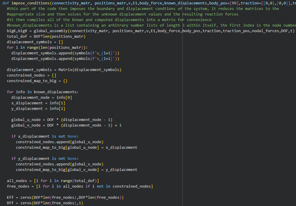
Impose Boundary Conditions
Solve for Unknown Displacements and Reaction Forces
Compute Stress and Strain
Loading and Boundary Conditions
The solver was developed to accommodate several types of structural loading, including distributed boundary tractions and concentrated nodal forces. Consistent element load vectors are generated from distributed loads using the Q4 shape functions, while concentrated forces are applied directly to their corresponding global degrees of freedom.
Essential boundary conditions can independently constrain either displacement component at selected nodes, allowing the program to represent rollers, fixed displacement directions, and combinations of displacement constraints.
This structure allows the same finite element routines to be reused for different geometries, meshes, loading conditions, and support configurations without modifying the underlying element formulation.
Verification and Validation
A dedicated verification study was performed to determine whether the independently developed solver reproduced the behavior predicted by commercial finite element software.
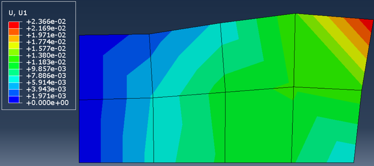
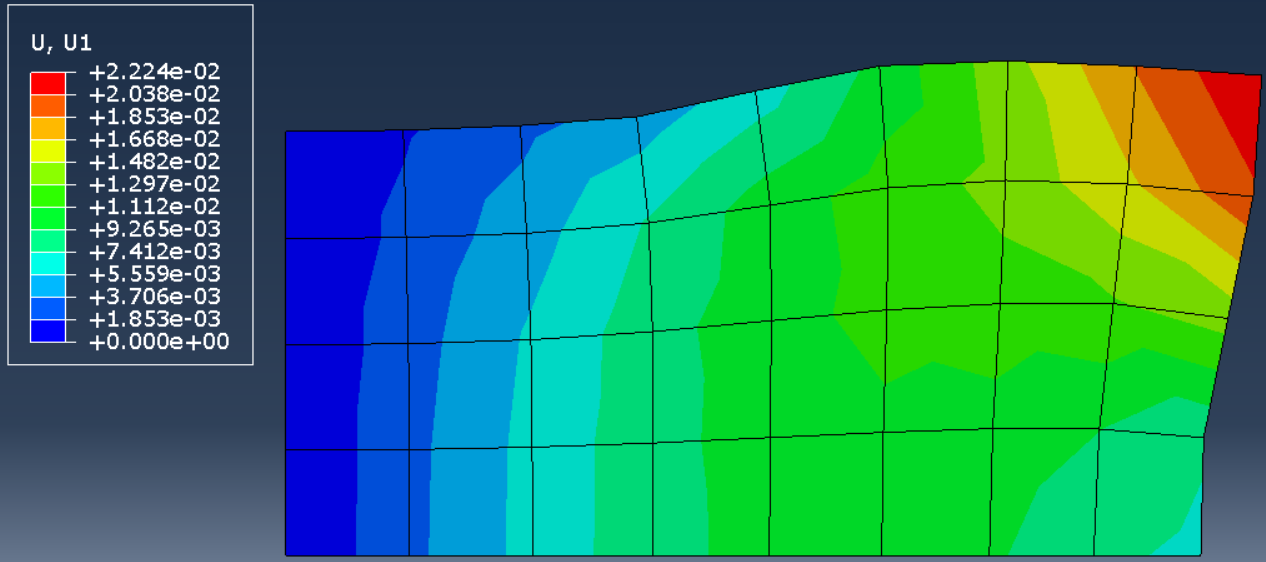
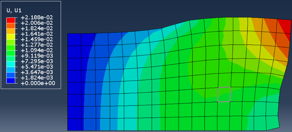
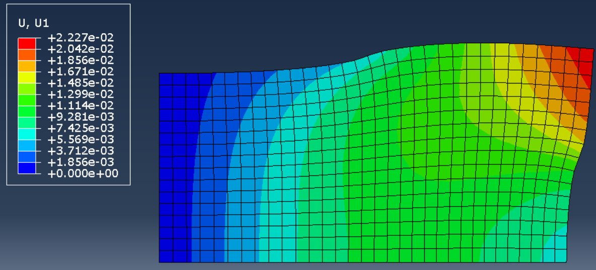
Equivalent plane-strain models were constructed in Abaqus/Standard using CPE4 quadrilateral elements with matching geometry, material properties, thickness, loading, and displacement boundary conditions.
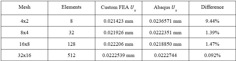
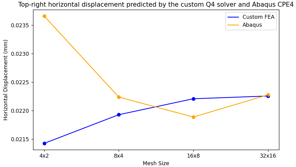
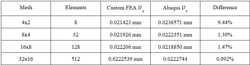
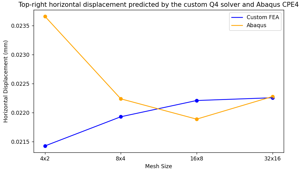
Initial comparisons using very coarse meshes produced noticeable differences between the two programs. Rather than modifying the custom solver simply to reproduce the Abaqus result, a systematic mesh-refinement study was performed to determine whether both formulations converged toward the same continuum solution.
The horizontal displacement of the top-right corner was selected as the comparison metric.
The two independently generated solutions converged as the mesh was refined. At 512 elements, the custom solver predicted a horizontal displacement within approximately 0.1% of Abaqus.
This verification provided strong evidence that the implemented element formulation, coordinate transformation, stiffness assembly, boundary-condition treatment, loading, and global solution procedure were functioning correctly.
Engineering Takeaways
The project provided experience with the complete computational process underlying commercial finite element software rather than treating FEA as a black-box analysis tool. Particular emphasis was placed on translating continuum mechanics and finite element equations into a reusable computational framework.
The verification process also demonstrated the importance of mesh convergence and numerical verification. A disagreement between two coarse-mesh solutions did not necessarily indicate an implementation error; progressively refining the discretization provided a more meaningful test of whether the independently implemented numerical methods approached the same physical solution.
The final comparison of 0.092% difference from Abaqus demonstrated successful implementation of the Q4 plane-strain formulation while also illustrating why verification should extend beyond comparison of a single finite element model.
Tools & Skills: Python • SymPy • NumPy • Abaqus • modular scientific programming • Q4 isoparametric elements • plane-strain elasticity • shape functions • Jacobian transformations • strain-displacement matrices • constitutive matrices • Gaussian quadrature • global stiffness assembly • stress/strain recovery • mesh convergence